Sentence Vectors with various techniques: TF-IDF, LSA and Deep Learning, Spatially visualizing sentence vectors; With Python Code

#AI-excercise #ai #Excercise

Comparing sentence vectors is interesting AI Exercise. This article takes text input, process it, and use three kinds of representations of the text data and does visualization of sentences in these three kinds of representations. The three kind of representations coved in this article are:

1. Tf Idf

2. Latent Semantic Analysis

3. Sentence Vector using DeepLearning

Sentences in big or even moderate-sized text files are quite sparse and plotting them in space is not very easy at times. Imagine you need to plot the sentences on the graph. This can be challenging especially because data turns out to be sparse and especially the projections are null in many dimensions. 

Let us understand a short to a medium-sized text file and visualize the sentences in lower dimensions, for now in x-y plane. 

The steps are given as follows, code with comments is given at end of steps

1. Take the text file and 

Load the individual sentences in a vector. Here climate change file was taken here are the initial sentences 

[‘\n’, ‘What Is Climate? How Is It Different From Weather?\n’, ‘You might know what weather is. Weather is the changes we see and feel outside from day to day. \n’….

The following sentences taken from article are studied here

Sentence[1]: What Is Climate? How Is It Different from Weather?

Sentence[10]: Different places can have different climates.

2. Convert the tf_idf file using fit_transform method  in python

Here is the snippet of sparse data in tf_idf

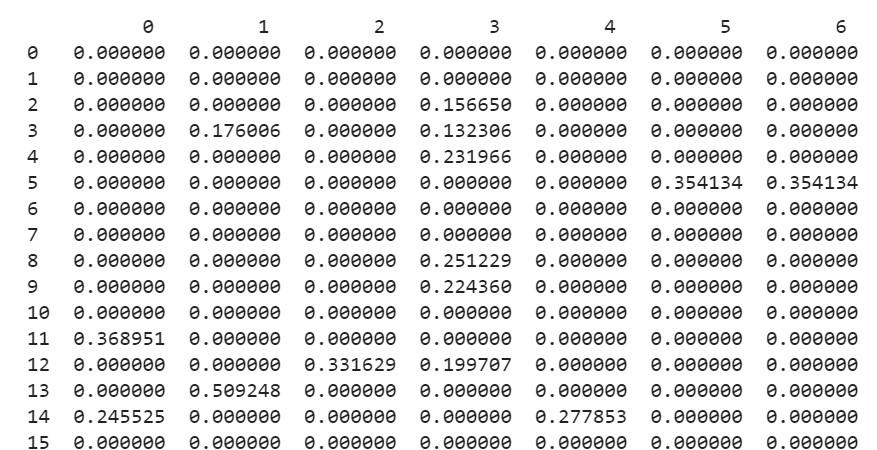
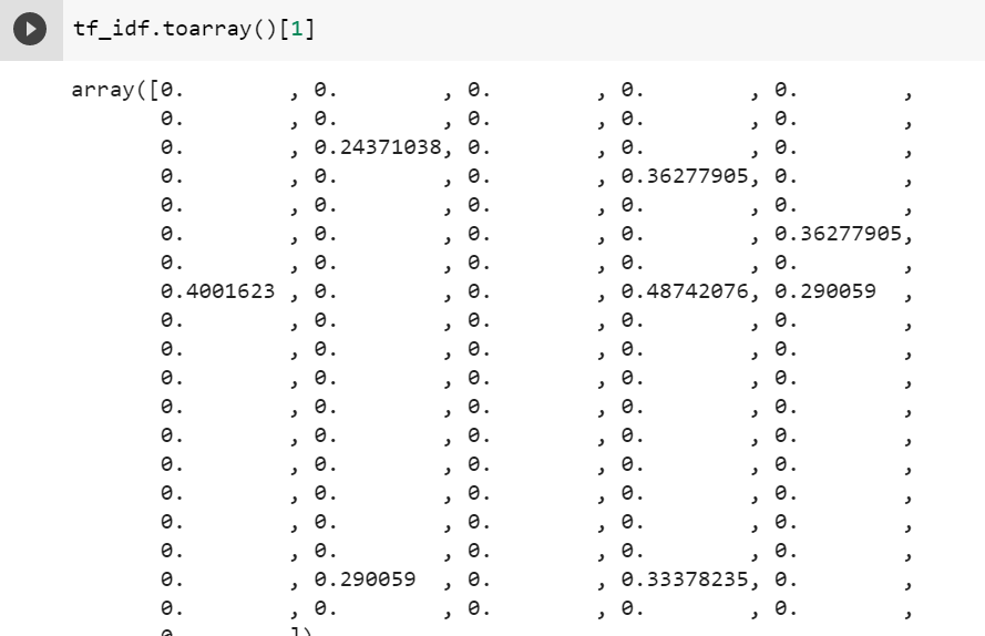
Sentence[1] representation in detail is as follows. Note this is sparse.

Now let us do the SVD of this data. This makes it ready for latent semantic analysis. The matrix U have the concepts with which sentences are represented.

M = U. S. VT [Basics of SVD in another article]

Let us view the matrix U here,

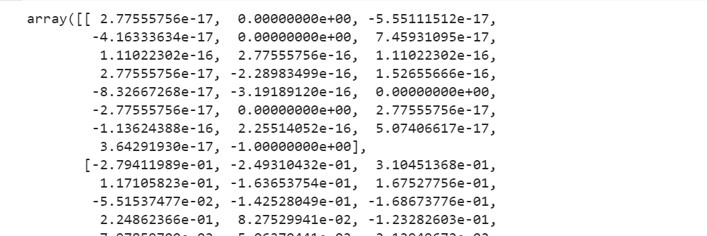
3. Choosing the second and eleventh sentence for visualizations on projection on xy-plane

Note-Indexing starts from 0 here, hence sentence[1] is the second sentence.

Sentence 2= array([-2.79411989, -2.49310432])

Sentence 11= array([-0.60383233, -1.66940253])

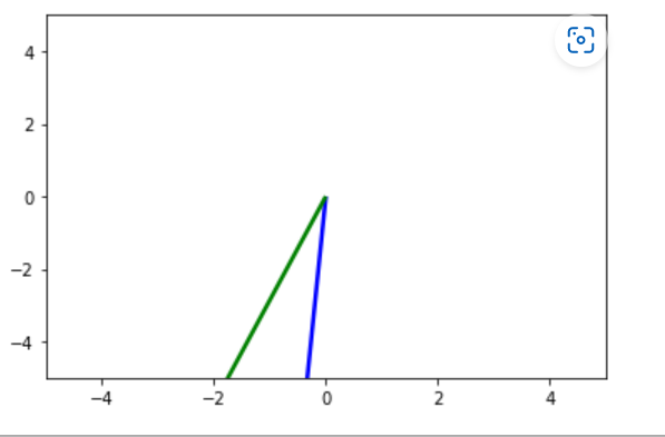
Pictorial Visualization of the LSA representation are as follows:

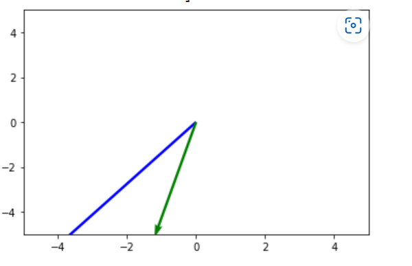
Plotting these two selected sentences from tf_idf representation gives the following graph.

4. Use Sentence Vectors using Deep Learning (BERT) to represent the text data. The following are projections on xy-plane.

2nd  sentence

array([-0.01798571, -0.1763664 ], dtype=float32)

11th  sentence

array([-0.07490239, -0.13899253], dtype=float32)

Similarity between these two chooses sentences

1. With Sentence Vectors truncated on xy plane

0.07610

2. Without truncation in Sentence Vectors

0.04472

3. With LSA 0.1201
4. With original data tf_idf 0.7625

Python Code here

import pandas as pd 

from sklearn.feature_extraction.text import TfidfVectorizer

import numpy as np

import matplotlib.pyplot as plt

pip install sent2vec

from sent2vec.vectorizer import Vectorizer

#read the sentences

sentences  = []

inputMediumfile = open("/content/CLIMATE_CHANGE1.txt")

for sentence in inputMediumfile:

  sentences.append(sentence)

print(sentences) 

#Use tf-idf on text data

vec = TfidfVectorizer()

tf_idf =  vec.fit_transform(sentences)

#Lets do the SVD of this data 

U,S,Vt = np.linalg.svd(tf_idf.toarray())

# Choosing the second and eleventh sentence

sen1 = U[:,:2]

vector1= sen1[1]

sen2 = u[:,:2]

vector2 = sen2[10]

#use Word and Sentence Embedding to get the representations

Vect = Vectorizer()

vect.run(sentences)

sentVectors = vect.vectors

More in next article