In this article, we propose to predict the preferred working hours by individuals based on the present inputs provided. Why this is required? As the work is preset and work goals are made based on resource predictions. Employees are resources of an organization and if we accumulate current phenomena with time we can predict well what shall be a pattern and hence work can be planned. These are independent of the organization a person works in. All data can be used in the entire country, which is selected. It lays emphasis that the pattern is followed in a demographic region rather than in an organization alone. The demographic region can be the entire Earth as well, but to start with country wise analysis can be made. Those employees who can fill in past data forms, this shall be even better. The form to be filled by employees is simple and does not need much time to fill. The form entries are the features of the RNN model we shall build. Hints of python code are provided here in the article.

The use of GRU lies in the fact that the data shall be stored in a historical format, hence we can predict say 6 months in advance, what the choices of people to work shall be. This can make the judgment to hire extra employees more clear to the organization.

At the same time, allowing flexible work, lesser or more, shall always benefit the employees. Tools like this can help both employees have the life balance they need and at the same time, work is not hampered.

The form to fill which is data to feed in the GRU is based on the following feature values:

1. Longitude
2. Latitude
3. Height
4. Weight
5. Income
6. Age
7. Gender
8. Working Hours
9. Type Of Work
10. Health
11. Num Children
12. Married Relationship
13. Nuclear family
14. Diet Veg NonVeg
15. GMT
16. Date
17. Month
18. Year

The target feature in this supervised learning is

1. Preferred Number of Working Hours

Here are some code snippets to explain the code of this Exercise. It’s on a dummy data, for now.

Note: No data was collected hence dummy data was used in the illustration exercise, for someone who has data to work on this exercise.

import pandas as pd

df = pd.read_excel('/content/woking_hours.xlsx')


print(df)

The output yields on a sample dummy data file are:

The data was observed once per candidate in six months. Total candidates are x, say 500 to start with.

If we want to predict the next six months ahead of time, the data is shifted by 30*6 observation points. After that new entries are made for the same candidates in order.

However, the data is not continuous, all values per candidate are not there. The look-ahead can be experimented with and learned with time. look_ahead to be changed as per requirements of modeling.

shift_data = 15

target_names = ['NoHours']
df_targets = df[target_names] 


df_targets = df[target_names].shift(-shift_data)

feature_names = [ 'GMT','D', 'M','Y', 'LAT',  'LONG' , 'Weight', 'Income', 'Age', 'Gender', 'WorkingHours', 'TypeOfWork', 'Health', 'NumChildren' ,'Married', 'Relatationship', 'Nuclear family', 'DietVegNonVeg']
df_feature  = df[feature_names] 

x_data = df_feature.values[0:-shift_data]
y_data = df_targets.values[0:-shift_data]


x_train, x_test, y_train, y_test=train_test_split(x_data, y_data, test_size=0.15)

num_x = x_data.shape[1]
print(num_x)

num_y = y_data.shape[1]
print(num_y)

model2 = Sequential()
model2.add(GRU(units=512,
              return_sequences=True,
              input_shape=(None, num_x)))

model2.add(Dense(num_y, activation='sigmoid'))


optimizer = RMSprop(lr=1e-3)
model2.compile(loss='mse', optimizer=optimizer)

model2.summary()

The output looks like-

.

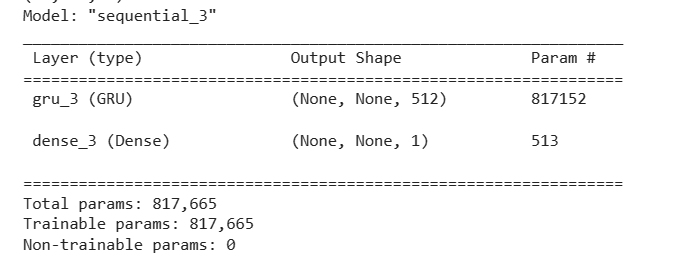
Fitting the Model

def batch_generator(batch_size, sequence_length):
 
    while True:
        x_type = (batch_size, sequence_length, num_x)
        x_batch = np.zeros(shape=x_type, dtype=np.float16)
        y_type = (batch_size, sequence_length, num_y)
        y_batch = np.zeros(shape=y_type, dtype=np.float16)

        for i in range(batch_size):
            i = np.random.randint(num_train - sequence_length)
            x_batch[i] = x_train[i:i+sequence_length]
            y_batch[i] = y_train[i:i+sequence_length]        
        yield (x_batch, y_batch)

batch_size = 50
sequence_length = 30 * 1
sequence_length

generator = batch_generator(batch_size=batch_size,
                            sequence_length=sequence_length)

model2.fit(x=generator,
           epochs=100,
           steps_per_epoch=50,
          validation_data=validation_data)

Evaluating Model

result = model2.evaluate(x=np.expand_dims(x_test, axis=0),
                        y=np.expand_dims(y_test, axis=0))

print("loss is", result)

Predicting

x  = x[0:end]
y  = y[0:end]
x = np.expand_dims(x, axis=0)
y_pred = model2.predict(x=x)

Note: This is a basic implementation as to implement this one needs the data and the rest of the things in this code can be fine-tuned.

The things to be fine-tuned are as follows:

1. The intervals of the shift to predict, right now 6-month steps.
2. The epochs and steps per epoch
3. Exact shape of input
4. Target values along with salary components
5. Determining the features of input entered by a user
6. MSE is used here, we need better error correction
7. Scaling was not performed, scaling of input and output needs to be performed for better optimized loss