Note: This same article appears in my median.com account as well

If you are new to AI or deep learning, here is your first CNN, or for now deep learning code.

Q. Why IRIS data?

A. As everyone is familiar with Iris data by now, so why not start with IRIS data. Too basic for CNN for sure, but too easy it would be then to understand and get to indepth with.

Though know IRIS data is too small for complex process such as deep learning, still it a good way to start to understant deep learning from the basic data set we all used as a first data science example. Simple, short and easy.

Here is a quick description with entire code required to do this.

Let’s import some good packages

import matplotlib.pyplot as plt
import tensorflow as tf
import numpy as np
import pandas as pd
import os
import math

from tensorflow.keras.layers import Input,  Embedding
from tensorflow.keras.backend import square, mean
from tensorflow.keras.models import Sequential
from tensorflow.keras.layers import InputLayer, Input
from tensorflow.keras.layers import Reshape, MaxPooling1D
from tensorflow.keras.layers import Conv1D, Dense, Flatten
from sklearn.preprocessing import MinMaxScaler
from sklearn.model_selection import train_test_split

Here is a snippet of data

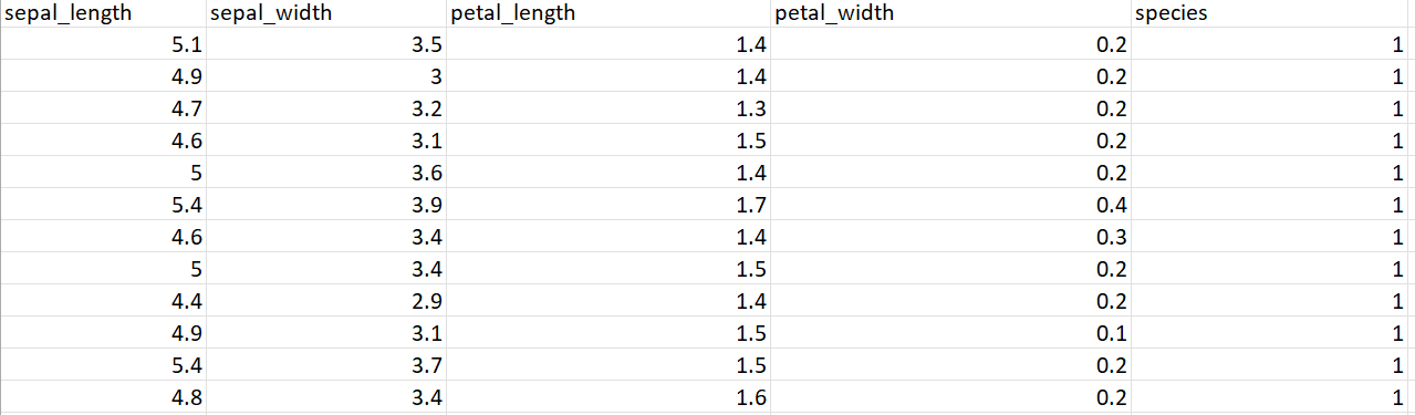
Lets us read this data in a data frame

df = pd.read_excel('/content/IRIS_Edited.xlsx')

print(df)

Read As

Read the features

feature_names = [ 'sepal_length','sepal_width', 'petal_length','petal_width']
feature  = df[feature_names] 
 
target_names = ['species']
targets = df[target_names]

x_data = feature.values 
y_data = targets.values 

Fit data, scale data and validate the data

x_train, x_test, y_train, y_test = train_test_split(x_data, y_data, test_size=0.15)

x_scaler = MinMaxScaler()
x_train_ = x_scaler.fit_transform(x_train)
x_test_ = x_scaler.transform(x_test)

y_scaler = MinMaxScaler()
y_train_ = y_scaler.fit_transform(y_train)
y_test_ = y_scaler.transform(y_test)

Make the CNN model

model = Sequential()
model.add(Conv1D(64, 2, activation="relu", input_shape=(4,1)))
model.add(Dense(4, activation="relu"))
model.add(MaxPooling1D())
model.add(Flatten())
model.add(Dense(3, activation = 'sigmoid'))
model.compile(loss = 'mse', 
     optimizer = "adam",               
              metrics = ['mse'])
model.summary()

Here is the model and the parameters

Find the result viz. accuracy

model.fit(x_train_, y_train_, batch_size=16,epochs=100)

result = model.evaluate(x=x_test_,
                        y=y_test_)

print("\n\nResult:", result)

Here are the traning and testing resuts, loss and mse

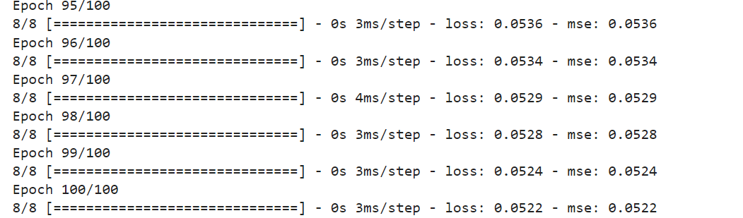
This leads to Result with a loss and mse as 0.0372. This result can be further analysed from various angles, explained in coming articles.